ALICE (A Large Ion Collider Experiment) is the LHC (Large Hadron Collider) experiment devoted to investigating the strongly interacting matter created in nucleus-nucleus collisions at the LHC energies. The ALICE ITS, Inner Tracking System, consists of six cylindrical layers of silicon detectors with three different technologies; in the outward direction: two layers of pixel detectors, two layers each of drift, and strip detectors. The number of parameters to be determined in the spatial alignment of the 2198 sensor modules of the ITS is about 13,000. The target alignment precision is well below 10 micron in some cases (pixels). The sources of alignment information include survey measurements, and the reconstructed tracks from cosmic rays and from proton-proton collisions. The main track-based alignment method uses the Millepede global approach. An iterative local method was developed and used as well. We present the results obtained for the ITS alignment using about 10$^5$ charged tracks from cosmic rays that have been collected during summer 2008, with the ALICE solenoidal magnet switched off.
JINST 5 (2010) P03003
e-Print: arXiv:1001.0502 | PDF | inSPIRE
CERN Record
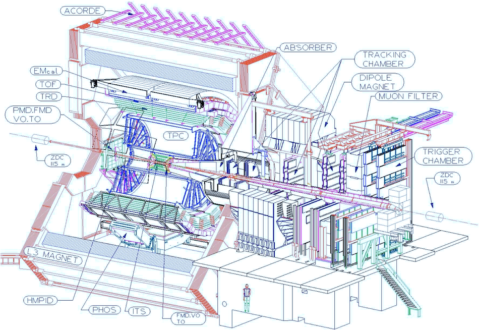
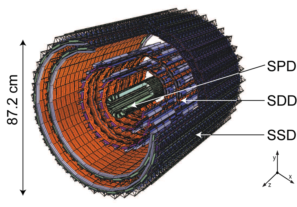


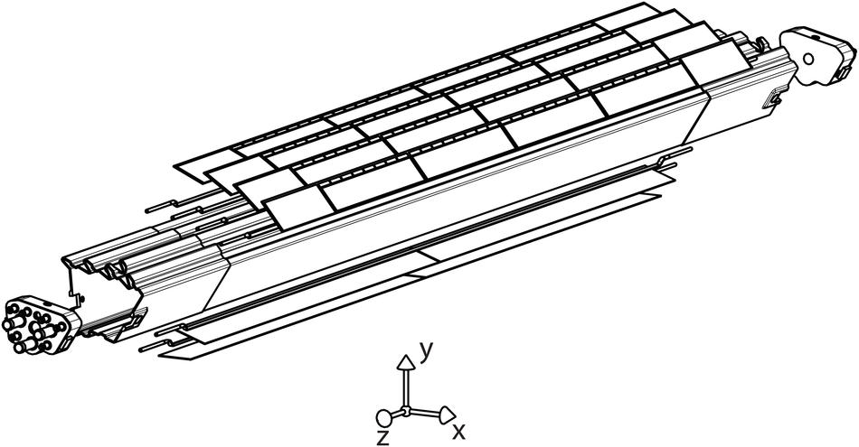


Figure 8
SSD survey validation. Top: distribution of $\Delta x_{\rm loc}$, the distance between two points in the module overlap regions along $z$ on the same ladder Bottom: distribution of the $r\varphi$ residuals between straight-line tracks defined from two points on layer 6 and the corresponding points on layer 5 In both cases, gaussian fits to the distributions with survey applied are shown (in top panel the fit range is $\pm2\,\sigma$, i.e $[-60 \mathrm{\mu m},+60 \mathrm{\mu m}]$). |   |
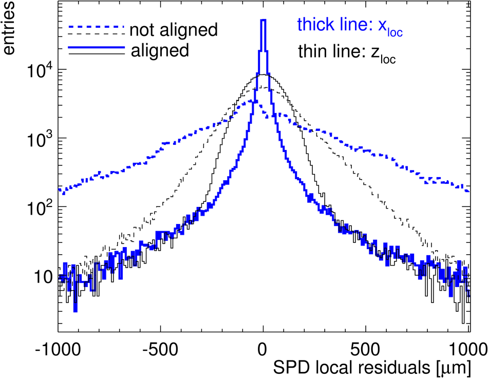

Figure 10
Top: distribution of $\Delta xy\vert_{y=0}$ for SPD only, before and after alignment Bottom: distribution $\Delta xy\vert_{y=0}$ for track segments reconstructed in the upper and lower parts of SPD+SSD layers;each track segment is required to have four assigned points; SSD survey and Millepede alignment corrections are applied. In both cases,the distributions are produced from the sample of events used to obtain the alignment corrections. |  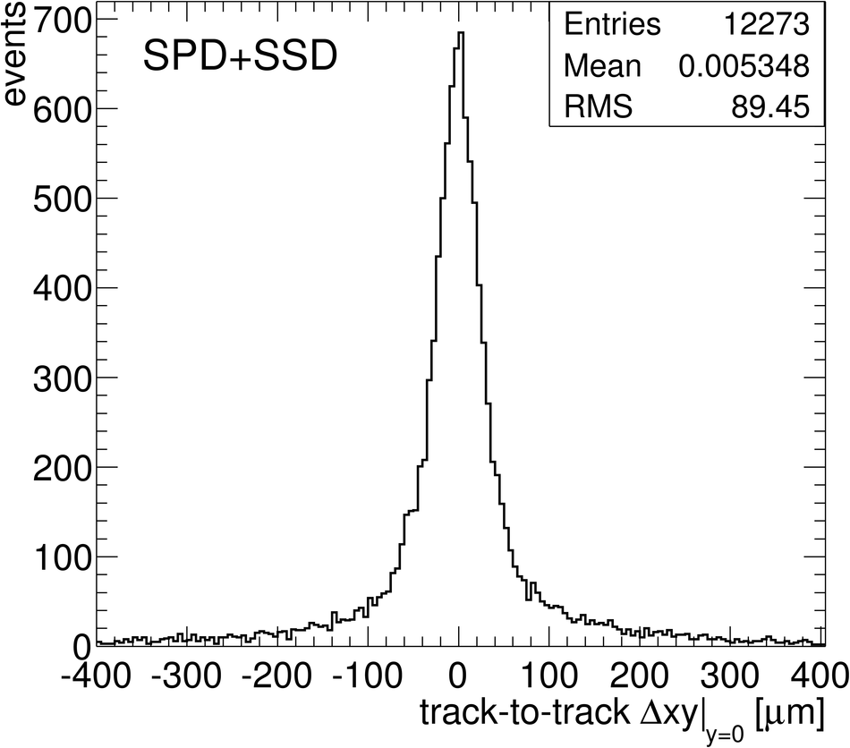 |
Figure 11
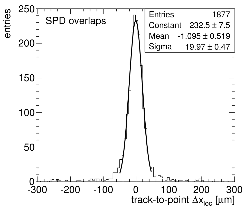
SPD double points in acceptance overlaps. Left:track-to-point $\Delta x_{\rm loc}$ for ``extra'' points before and after alignment Right: $\sigma$ of the $\Delta x_{\rm loc}$ distributions as a function of thetrack-to-module incidence angle selection; 2008 cosmic-ray data are compared to the simulation with different levels of residual misalignment See text for details. | 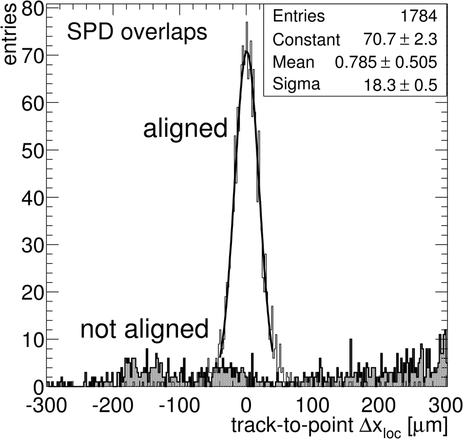  |
Figure 12
Alignment stability tests Top: for SPD only, distribution of the $\Delta xy\vert_{y=0}$ distance obtained when aligning with every second track and checking the alignment with the other tracks Bottom: track-to-point residuals in the inner SPD layer (track fit in outer SPD layer and in the two SSD layers), for $\rm B=0$ and $\rm B=\pm 0.5 T$ (the three histograms are normalized to the same integral). | 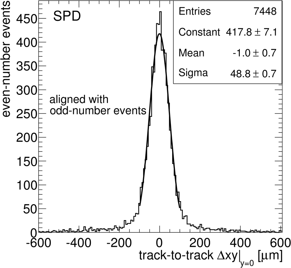 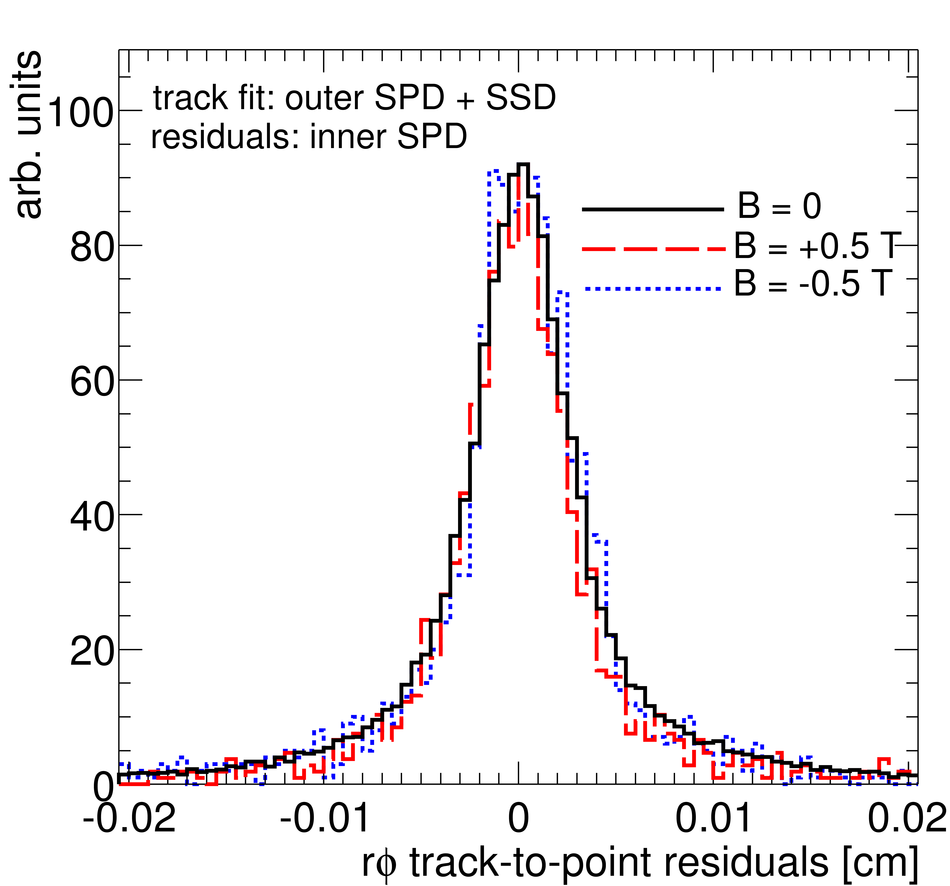 |
Figure 13
SDD calibration and alignment Top: distribution of track-to-point residuals in the two drift regions for the SDD modules of layer 4 side C ($z< 0$); tracks are fitted using only their associated points in SPD and SSD; the Millepede alignment corrections for SPD and SSD are included, as well as the SSD survey Bottom: residuals along the drift coordinate for one SDD module as a function of drift coordinate after Millepede alignment with only geometrical parameters and with geometrical+calibration parameters. | 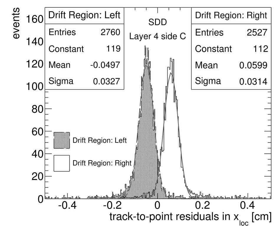  |